How a Single Equation Powers Crypto Exchanges

Do you remember the Crypto BOOM of 2021-2022? There were a lot of tokens, NFTs, and crypto exchanges coming up, showing millions of dollars of trade. NFTs — yeah, those apes’ images — were selling for thousands of dollars alone. That time I was exploring these new Platforms and learning Web3 and Solidity. I got to know about Decentralized Crypto Exchanges or DEX for short.

You might have heard about or maybe even used — Uniswap or Pancake swap. DEXs work differently from traditional Crypto Exchanges like Binance/Robinhood. Traditional Exchanges are Centralized, which means that your funds are managed by them or in other words they are an intermediary between traders. To facilitate trades they use Order Book. DEXs work differently — there are no intermediaries on DEXs, rather trades are facilitated by Code and Math.

Around that time, I wanted to implement a DEX from scratch on my own, everything from Math to Code! You can view a demo at https://dex-web-krishbaidya.vercel.app/ (DO NOT make a transaction you may lose money)

In this post, we are going to look at AMM — Automated Market Maker, the Math behind them, and explore some code.

What Do We Need to Find?

We need to find a general formula for current price of one Token based on the amount of both the Tokens available.

Setting up the Stage

These are the required properties our DEX must follow:

Token conservation

We cannot just make new Tokens. The total amount of both, let’s say USDT and ETH, in the system must be the same before and after a transaction. This ensures that we are not creating any new tokens and are compatible with external contracts such as tokens contract itself.

K stays constant

The proportional relationship between the two tokens must remain the same after every trade. If the pool has more USDT, it must have less ETH to compensate — and vice versa. This balance is enforced by a constant we’ll call k .

Reversibility

This property is interesting. We can do the transactions in just the reverse order to get to previous state. Here’s a simple example -

1. Let’s say the DEX has 100 USDT and 100 ETH tokens.
2. User does a BUY transaction of 10 USDT to get some ETH.
3. Now if the user does a SELL transaction of those ETH, they will get 10 USDT back and the state of DEX goes back to 100 USDT and 100 ETH.

Note — in real DEX this usually does not happen because of transaction fees.

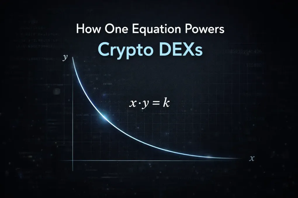
The AMM formula

So now how should our formula look like? We know that as x increases, y must decrease — and vice versa. That’s an inverse relationship, which in math looks like this:

Derivation

where x,y are amount of tokens A and B and k is proportionality constant.

In our DEX, x is the USDT reserve, y is the ETH reserve, and k remains constant during swaps, but changes when liquidity providers add or remove liquidity.

This formula alone doesn’t tell us how much the price changes per trade, so we extend it to include token amount variation:

Similarly for $\Delta x$:

We now have a formula that tells you how much to change Token A to compensate for change in Token B .

Example with Code

Let’s see how this plays out in Python — we’ll run a round-trip trade and verify all three properties hold.

Setup Initial liquidity pool

# The pool starts with equal reserves of both tokens.
# k is the invariant — it must never change between trades.
_x = 100   # USDT reserve
_y = 100   # ETH reserve
_k = _x * _y  # initial k (changes if liquidity changes)

Core math Price discovery — how much ETH for Δx tokens?

def get_token_price(token_amount: int) -> float:
    """
    Given a USDT amount to buy, returns how much ETH must be paid.
    Derived from: (x - Δx)(y + Δy) = k
    So:           Δy = k / (x - Δx) - y
    """
    assert _k > 0,            "Pool has no liquidity"
    assert token_amount > 0,  "Must buy a positive amount"
    assert token_amount < _x, "Cannot drain the pool"

    new_x = _x - token_amount        # pool loses USDT
    new_y = _k / new_x               # k stays constant → y must rise
    eth_cost = new_y - _y            # trader pays the difference
    return eth_cost

def get_eth_price(eth_amount: int) -> float:
    """
    Given an ETH amount to sell, returns how much USDT is received.
    Derived from: (x + Δx)(y - Δy) = k
    So:           Δx = k / (y - Δy) - x
    """
    assert _k > 0,          "Pool has no liquidity"
    assert eth_amount > 0, "Must sell a positive amount"
    assert eth_amount < _y, "Cannot drain the pool"

    new_y = _y - eth_amount          # pool loses ETH
    new_x = _k / new_y               # k stays constant → x must rise
    usdt_out = new_x - _x            # trader receives the difference
    return usdt_out

Trades Buy and sell — update pool state after each trade

def buy(token_amount: int) -> float:
    """Buy USDT from the pool by paying ETH. Returns ETH paid."""
    global _x, _y
    eth_paid = get_token_price(token_amount)
    _x -= token_amount  # pool gives USDT to trader
    _y += eth_paid       # pool receives ETH from trader
    return eth_paid

def sell(eth_amount: int) -> float:
    """Sell ETH back to the pool. Returns USDT received."""
    global _x, _y
    usdt_received = get_eth_price(eth_amount)
    _y -= eth_amount      # pool gives ETH back
    _x += usdt_received   # pool receives USDT from trader
    return usdt_received

Demo Round-trip trade — proving reversibility

print(f"Initial state:  USDT={_x}  ETH={_y}  k={_k}")

# Step 1 — buy 10 USDT, pay ETH
eth_paid = buy(10)
print(f"Bought 10 USDT. Paid {eth_paid:.4f} ETH.")
print(f"Pool mid-state: USDT={_x:.4f}  ETH={_y:.4f}  k={_x*_y:.2f}")
print()

# Step 2 — sell that exact ETH amount back
usdt_back = sell(eth_paid)
print(f"Sold {eth_paid:.4f} ETH. Received {usdt_back:.4f} USDT.")
print(f"Final state:    USDT={_x:.2f}  ETH={_y:.2f}  k={_x*_y:.2f}")

Output What you’ll see

Initial state:  USDT=100  ETH=100  k=10000

Bought 10 USDT. Paid 11.1111 ETH.
Pool mid-state: USDT=90.0000  ETH=111.1111  k=10000.00

Sold 11.1111 ETH. Received 10.0000 USDT.
Final state:    USDT=100.00  ETH=100.00  k=10000.00

Conclusion & What’s Next?

So there we have it! We just proved how a simple middle-school math equation — $x \cdot y = k$ — can power a decentralized exchange and handle billions of dollars in trades, all without a single middleman or order book.

But… the real world is a bit messier than our perfect Python script.

If you look closely at the math, buying a massive amount of tokens from a pool shoots the price up drastically. This is called Slippage, and it protects the pool from being completely drained. Also, in our code, the trades were completely free. In reality, DEXs charge a small fee (usually around 0.3%) to reward the folks providing the liquidity, which means our constant k actually increases slightly over time!

And here is the biggest catch — providing tokens to these pools exposes you to a mathematically terrifying risk called Impermanent Loss, where you can actually lose money compared to just holding your crypto in a wallet.

But how do you solve a flaw built into the very math that makes the entire system work? Well… that’s a topic for another post! Until then, keep exploring and building!